Lab 10
Prelab
In this lab, we will be setting up a virtual model where we implement a Bayes filter to localize a virtual robot in a simulated 2D area. This simulator is meant to model a physical lab environment where there is a bounded room with walls and obstacles, where the robot can move and collect 18 readings per time step by rotating a full 360 degrees in place.
In-Class Exercises
Open Loop Control
I started out with open loop control, making the robot follow a set of velocity commands to turn in a square shape.
Here is the code, along with the car running and the ground truth and odometry being plotted alongside it.
while cmdr.sim_is_running() and cmdr.plotter_is_running():
    pose, gt_pose = cmdr.get_pose()
    cmdr.set_vel(0,1.5)
    time.sleep(1.05)
    cmdr.set_vel(0.8,0)
    time.sleep(0.5)
    cmdr.plot_odom(pose[0], pose[1])
    cmdr.plot_gt(gt_pose[0], gt_pose[1])
    sensor_values = cmdr.get_sensor()
What is the duration of a velocity command?
I made the robot turn for 1.05s, since the units are in radians/second and I set to turn at about 1.5 radians/second (~90 degrees). I then let the car run straight for 0.5s at 0.8m/s. Depending on how long each loop execution takes, it takes at least 1.55s for it to run.
Does the robot always execute the exact same shape?
No, since it doesn't turn at exactly 90 degrees, overtime the error compounds and the robot starts to move in a different shape.
Closed Loop Control
I now designed a simple closed loop controller that took in the distance from the wall and randomly decides to turn left or right.
import random
cmdr.reset_plotter()
cmdr.reset_sim()
direction = [-4, 4]
while cmdr.sim_is_running() and cmdr.plotter_is_running():
    pose, gt_pose = cmdr.get_pose()
    if cmdr.get_sensor() < 0.5:
        cmdr.set_vel(0,random.choice(direction))
        time.sleep(1)
    cmdr.set_vel(2,0)
    cmdr.plot_odom(pose[0], pose[1])
    cmdr.plot_gt(gt_pose[0], gt_pose[1])
    sensor_values = cmdr.get_sensor()
By how much should the virtual robot turn when it is close to an obstacle?
I decided to turn by 90 degrees using the same method as before. However, I did increase the speed for the robot to turn 4 radians/s compared to the previous 1.5 rad/s.
At what linear speed should the virtual robot move to minimize/prevent collisions? Can you make it go faster?
The faster I make the virtual robot go, the greater the distance it reads must be to turn in time. At a reading distance of 0.5m, the fastest I could make it reliably move was about 2m/s.
How close can the virtual robot get to an obstacle without colliding?
At 2 m/s, 0.3m was approximately the shortest distance that let the car successfully go towards the wall and turn.
Does your obstacle avoidance code always work? If not, what can you do to minimize crashes or (may be) prevent them completely?
Previously, I changed the car's velocity and minimum distance from the wall to turn. However, even after finding the right values for this, the robot would still graze past the boundary/objects.
One of the best ways to fix this would be if the distance measurement was not just a straight line, but a cone such that the robot does not graze by obstacles that is not detected in its limited stright line of sight.
Bayes Filter
The Bayes filter is an iterative two-phase algorithm. At each time step, the robot completes a motion and collects a new set of sensor readings. The filter processes this information in the following sequence:
- Prediction step where the motion model is integrated over every grid cell, given the previous belief $bel(x_{t})$ and the most recent control input $u_{t}$.
$$ \overline{bel}(x_{t}) = \Sigma_{x_{t-1}}p(x_{t}|u_{t}, x_{t-1}) \dot bel(x_{t-1}) $$
- Update
$$ bel(x_{t})= \eta \dot p(z_{t}|x_{t}) \dot \overline{bel}(x_{t}) $$
Compute Control
This function extracts the odometry motion triplet $(\delta_{rot1},\delta_{trans}, \delta_{rot2})$ from two consecutive poses. I use normalize_angle on both rotations to stay within [-180, 180).
def compute_control(cur_pose, prev_pose):
  dx = cur_pose[0] - prev_pose[0]
  dy = cur_pose[1] - prev_pose[1]

  heading = math.degrees(math.atan2(dy, dx))

  delta_rot_1 = mapper.normalize_angle(heading - prev_pose[2])
  delta_trans = math.hypot(dx, dy)
  delta_rot_2 = mapper.normalize_angle(cur_pose[2] - prev_pose[2] - delta_rot_1)

  return delta_rot_1, delta_trans, delta_rot_2
Odometry Motion Model
This function returns the transition probability p(x'|x,u) as the product of three Gaussians (one per odometry component), comparing the motion needed to connect the two poses against the motion actually observed.
def odom_motion_model(cur_pose, prev_pose, u):
  actual_rot1, actual_trans, actual_rot2 = u
  needed_rot1, needed_trans, needed_rot2 = compute_control(cur_pose, prev_pose)
  prob  = loc.gaussian(mapper.normalize_angle(needed_rot1 - actual_rot1),  0, loc.odom_rot_sigma)
  prob *= loc.gaussian(needed_trans - actual_trans,                         0, loc.odom_trans_sigma)
  prob *= loc.gaussian(mapper.normalize_angle(needed_rot2 - actual_rot2),  0, loc.odom_rot_sigma)
  return prob
Prediction Step of Bayes Filter
This loops over all previous and current cell pairs, accumulating weighted transition probabilities into $bel_bar$. Cells with belief below 0.0001 are skipped for speed.
def prediction_step(cur_odom, prev_odom):
  u = compute_control(cur_odom, prev_odom)
  loc.bel_bar = np.zeros((mapper.MAX_CELLS_X, mapper.MAX_CELLS_Y, mapper.MAX_CELLS_A))

  for cx_prev in range(mapper.MAX_CELLS_X):
      for cy_prev in range(mapper.MAX_CELLS_Y):
          for ca_prev in range(mapper.MAX_CELLS_A):
              prob_prev = loc.bel[cx_prev, cy_prev, ca_prev]
              if prob_prev < 0.0001:
                  continue

              prev_pose = mapper.from_map(cx_prev, cy_prev, ca_prev)

              for cx in range(mapper.MAX_CELLS_X):
                  for cy in range(mapper.MAX_CELLS_Y):
                      for ca in range(mapper.MAX_CELLS_A):
                          cur_pose = mapper.from_map(cx, cy, ca)
                          p = odom_motion_model(cur_pose, prev_pose, u)
                          loc.bel_bar[cx, cy, ca] += p * prob_prev
  loc.bel_bar /= np.sum(loc.bel_bar)
Sensor Model
This function broadcasts the 18 observed ranges against $mapper.obs_view$ using numpy, returning a Gaussian likelihood for every cell at once with no explicit loop.
def sensor_model(obs):
  prob_array = loc.gaussian(mapper.obs_views - obs, 0, loc.sensor_sigma)
  return prob_array
Update Step of Bayes Filter
This function multiplies $bel_bar$ by the per-cell sensor likelihood (product over the 18 measurements using $np.prod(axis=3)$) and renormalizes to get $bel$.
def update_step():
  obs = loc.obs_range_data.flatten()
  likelihood = np.prod(sensor_model(obs), axis=3)
  loc.bel = likelihood * loc.bel_bar
  loc.bel /= np.sum(loc.bel)
Results & Analysis
Trajectory Run:
First Run:
Other Runs:
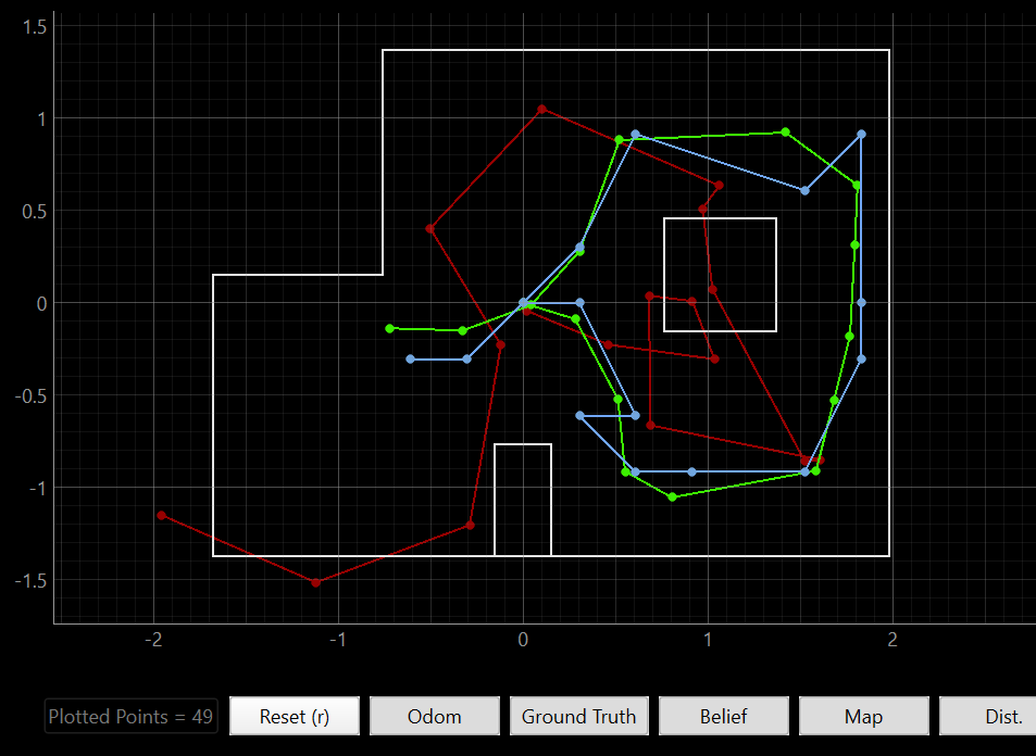
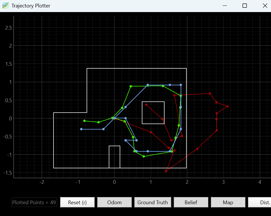
From these runs we can see how important the Bayes filter is. It is a massive improvement over raw odometry in both runs. Even in the worst run, the belief stays inside the map and follows the rough shape of the true trajectory. The remaining error is a natural consequence of the 30 cm grid resolution and the Gaussian approximation in both models.