Lab 2

In this lab we begin to work with our IMU and understand how to edit and analyze the accelerometer and gyroscope's output.

Prelab

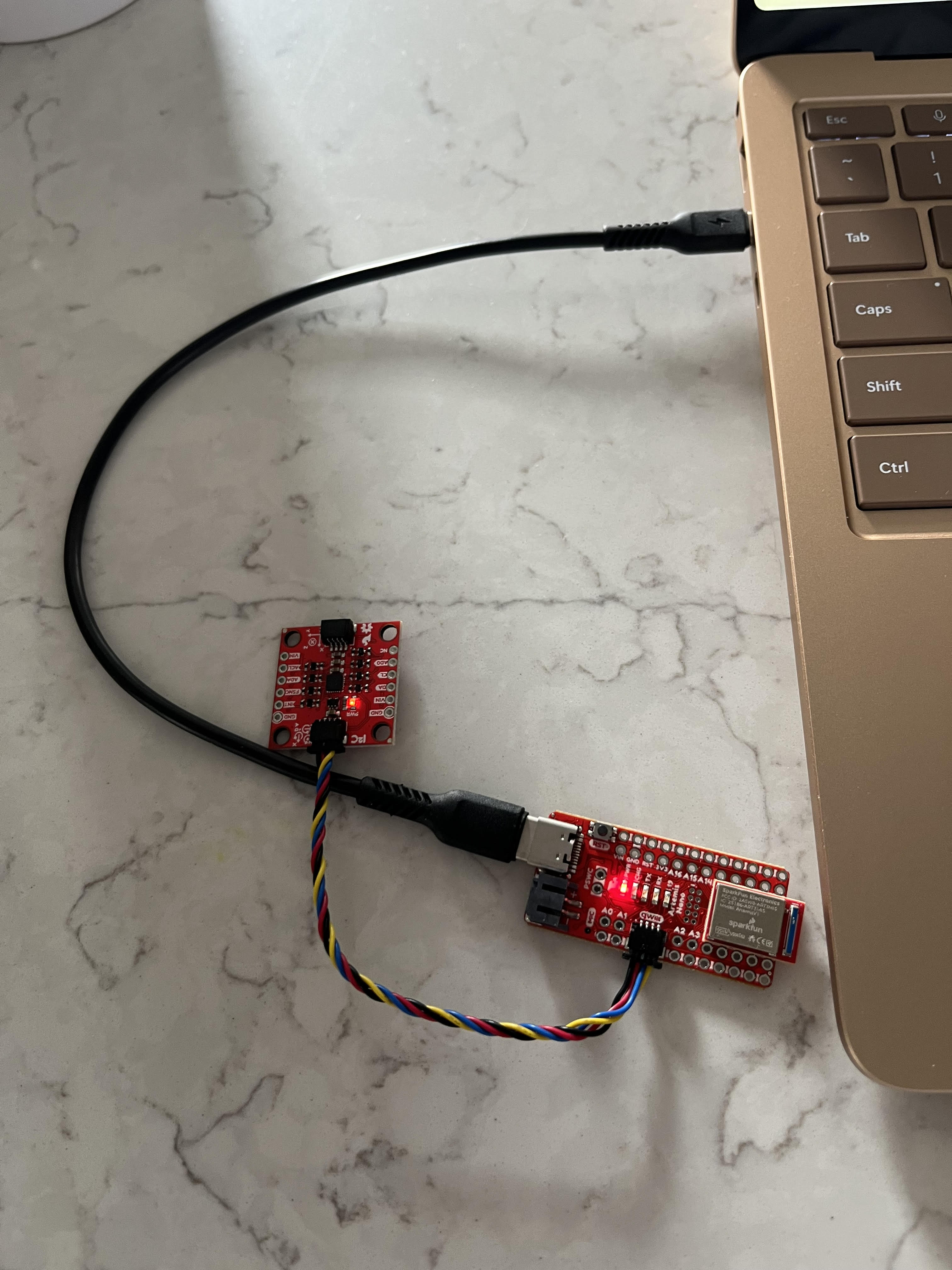
I installed the SparkFun 9DOF IMU Breakout_ICM 20948_Arduino Library in Arduino IDE, and connected the IMU to the Redboard Artemis Nano board via the QWIIC connectors as seen below.

Task 1 - Accelerometer

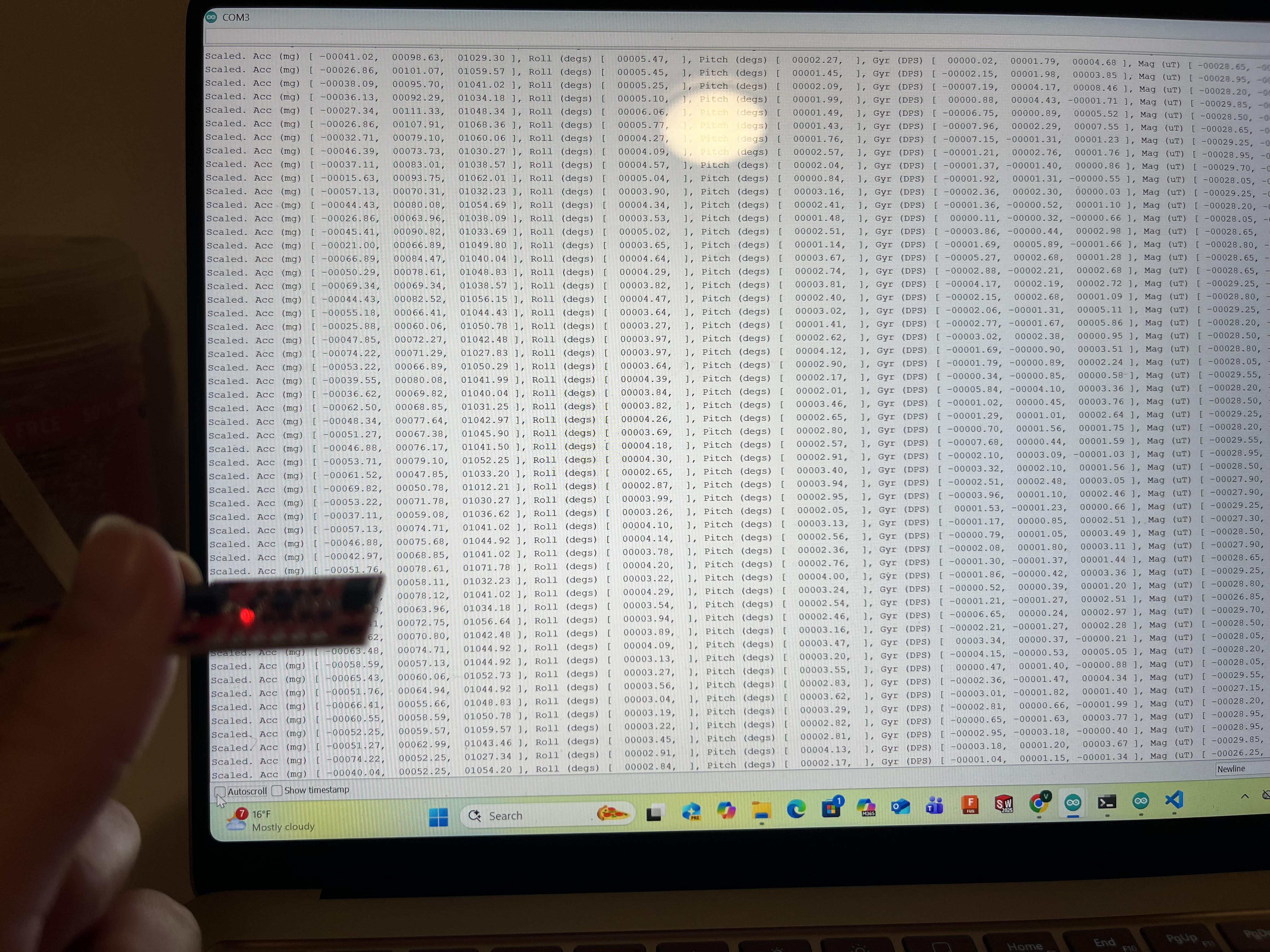
I started off by running the IMU data to see if it worked as shown below.

AD0_VAL is defined as 1 in the example code. This variable represents the last bit of the I2C address, and the value 1 means that it is always pulled high.

The accelerometer measures acceleration along each axis, the gyroscope measures rate of angular change along each axis in degrees per second, and the magnetometer measures Earth’s magnetic field. When the IMU is flat on my hand or table the accelerometer reads ~1000.00 in the z direction (the units are in mg), representing the acceleration of Earth’s gravitational field.

Soon after, I used the equations from class to calculate pitch and roll in degrees.

  SERIAL_PORT.print(" ], Roll (degs) [ ");
  printFormattedFloat((atan2(ay,az))*(180/M_PI), 5, 2);
  SERIAL_PORT.print(", ");
  SERIAL_PORT.print(" ], Pitch (degs) [ ");
  printFormattedFloat(atan2(-ax, sqrt(ay*ay + az*az)) * 180.0 / M_PI, 5 ,2);

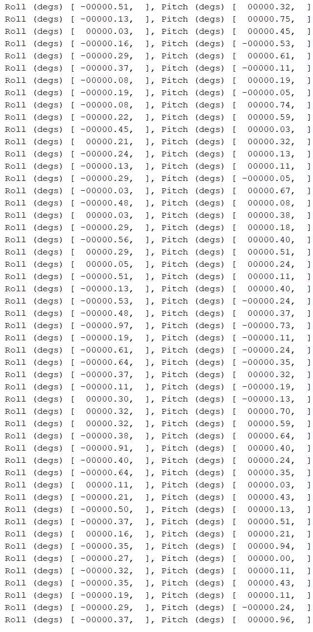
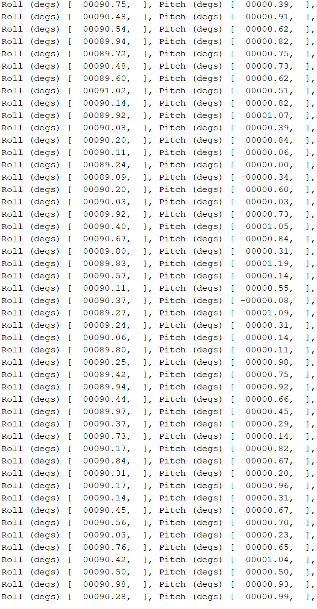
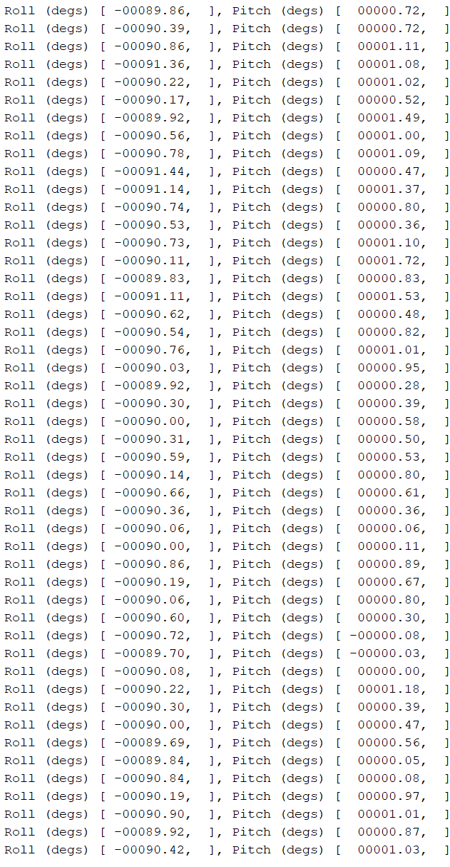
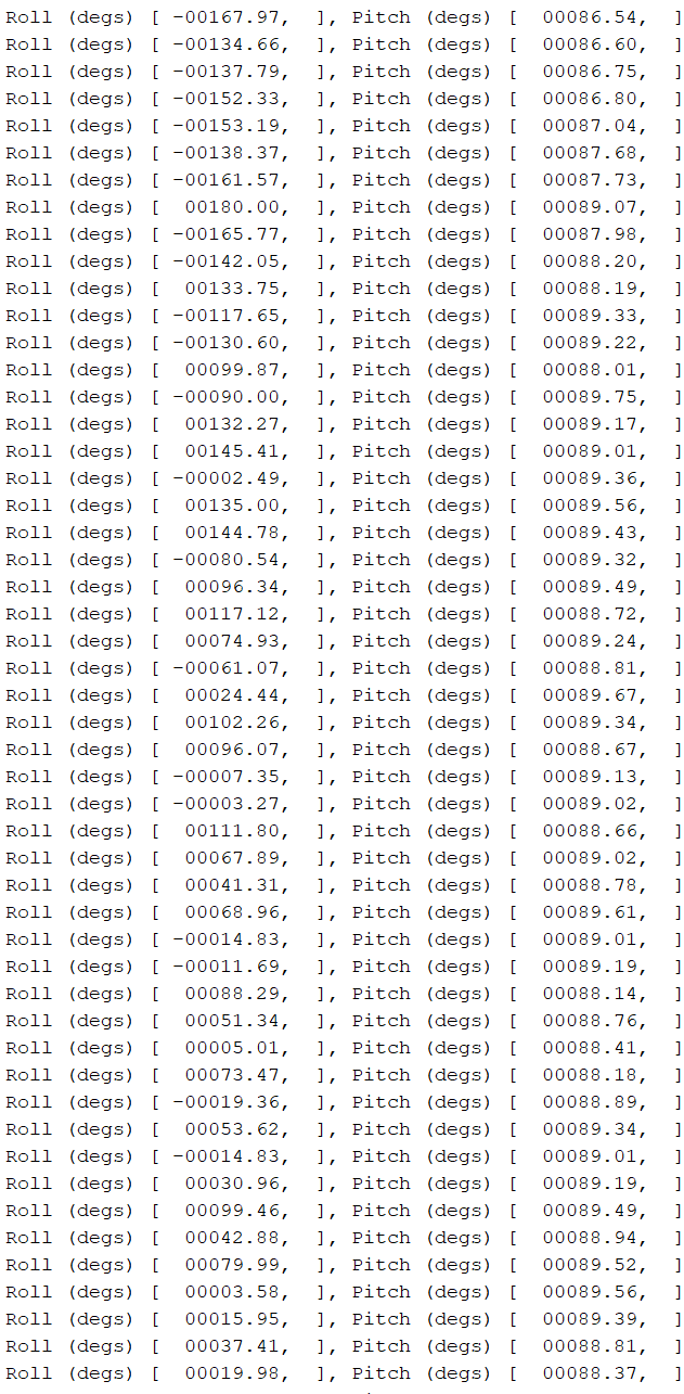
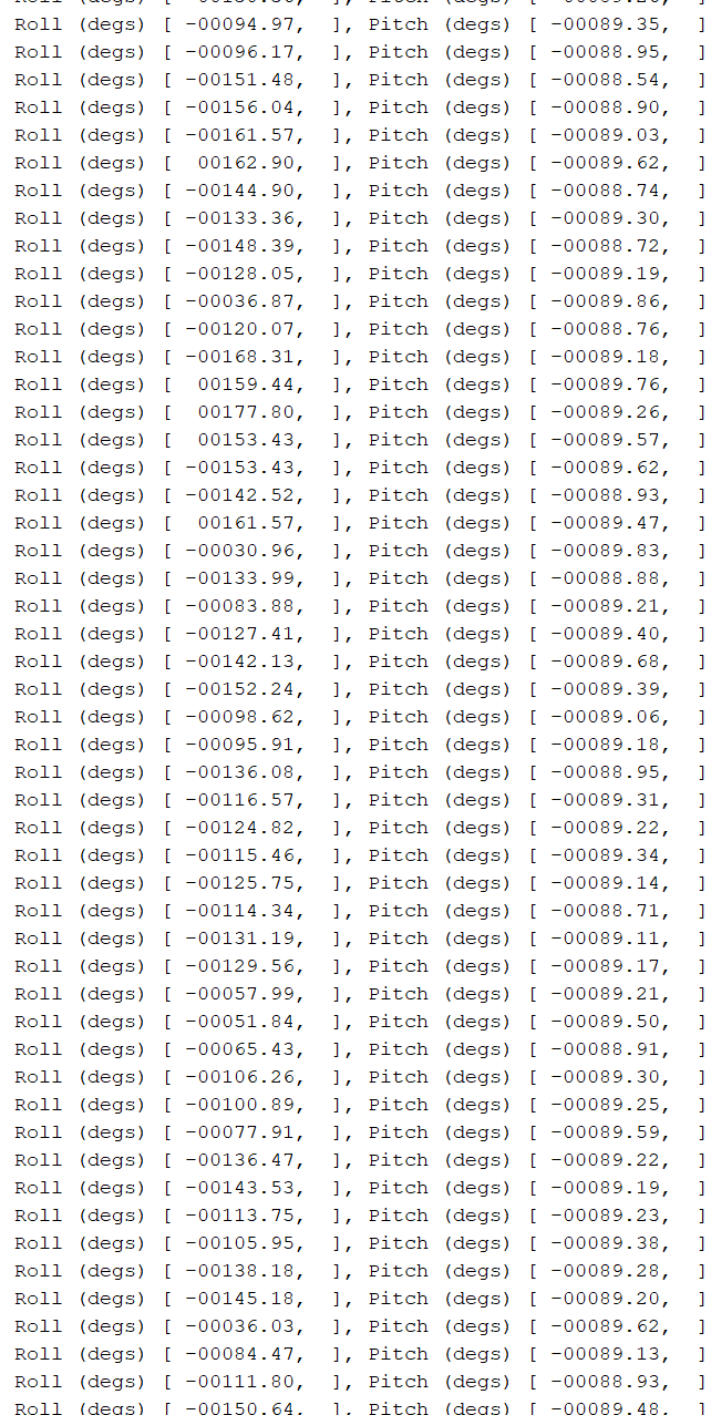
The following is a video, followed by photos of achieving -90, 0, 90 degrees in roll and pitch.

When I simply used the atan2 function for the pitch, I would not get zero when the IMU was flat on the table at rest. I used ChatGPT in order to problem solve, and ended up using the equation shown above which provided me with correct results.

The accelerometer was pretty accurate, I would never get a reading that deviated more than 1.5 degrees from what I expected it to be, therefore I did not perform any additional calibration method.

As for the noise, I decided to collect about 250 samples of the roll and pitch data and plot the data in the frequency domain as shown below:

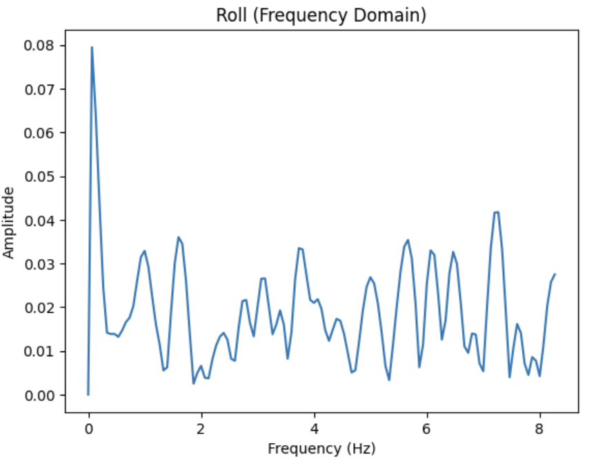
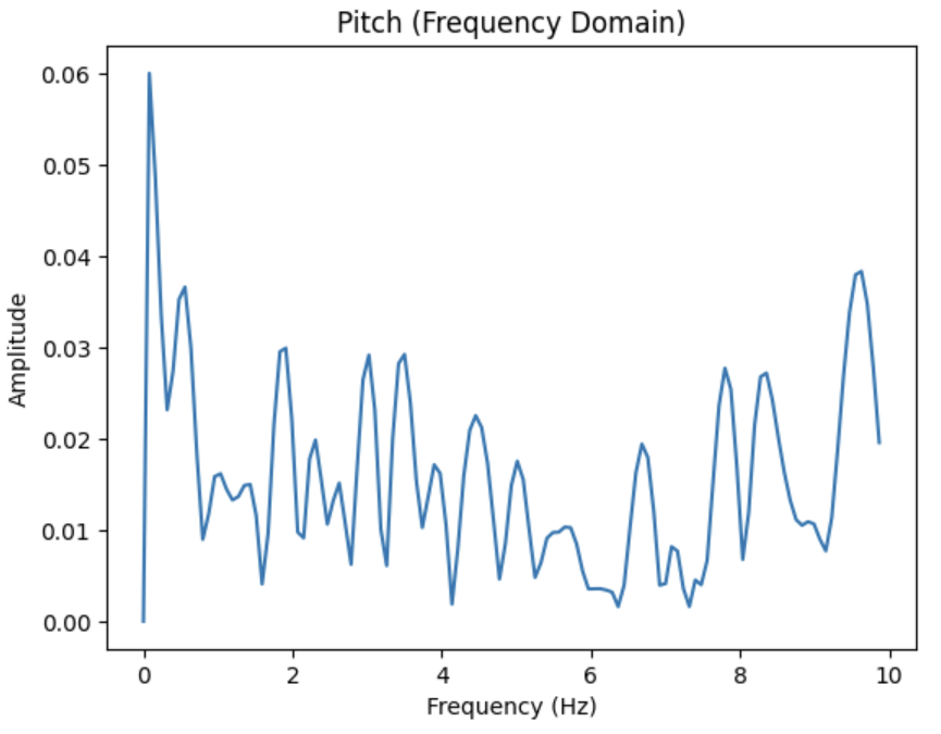
As we can see, both frequency plots seem to be abit noisy, but have a large peak at a low frequency of less than 0.25 Hz for both Roll and Pitch. A cutoff frequency above 0.25 Hz, about 0.5 Hz can help preserve the signal while filtering out the high frequency noise.

I created the plots using the code below:

import numpy as np
import matplotlib.pyplot as plt
from scipy.fftpack import fft


N = 250  # how many samples to read - got from Arduino code

t_ms = np.zeros(N)
roll = np.zeros(N)
pitch = np.zeros(N)

ble.send_command(CMD.senddataover, "")

for i in range(N):
    data = ble.receive_string(ble.uuid['RX_STRING']).strip()
    parts = data.split()
    t_ms[i] = float(parts[1])
    roll[i] = float(parts[3])
    pitch[i] = float(parts[5])

# ms -> seconds
t = t_ms / 1000.0

# Estimate sampling rate
dt = np.diff(t)
fs = 1.0 / np.mean(dt)
print("Estimated sampling rate (Hz):", fs)

def do_fft(signal, fs):
    signal = signal - np.mean(signal)  # remove DC
    N = len(signal)

    X = fft(signal)
    freq = np.fft.fftfreq(N, d=1/fs)

    half = np.arange(N//2)
    return freq[half], (2.0/N) * np.abs(X[half])

freq_roll, amp_roll = do_fft(roll, fs)
freq_pitch, amp_pitch = do_fft(pitch, fs)



plt.figure()
plt.plot(freq_roll, amp_roll)
plt.xlabel("Frequency (Hz)")
plt.ylabel("Amplitude")
plt.title("Roll (Frequency Domain)")
plt.show()

plt.figure()
plt.plot(freq_pitch, amp_pitch)
plt.xlabel("Frequency (Hz)")
plt.ylabel("Amplitude")
plt.title("Pitch (Frequency Domain)")
plt.show()

The code above calls on the following command:

case senddataover:{
    const int N = 250; // 250 samples
    float rollarr[N];
    float pitcharr[N];

    uint32_t startt = millis();

    for (int i=0; i<N; i++)
    {
        myICM.getAGMT();
        float timee = millis() - startt;
        float ax = myICM.accX();
        float ay = myICM.accY();
        float az = myICM.accZ();

        rollarr[i]  = atan2(ay, az) * 180.0 / M_PI;
        pitcharr[i] = atan2(-ax, sqrt(ay*ay + az*az)) * 180.0 / M_PI;
        tx_estring_value.clear(); 
        tx_estring_value.append("Time: ");
        tx_estring_value.append(timee);
        tx_estring_value.append(" ROLL: ");
        tx_estring_value.append(rollarr[i]);
        tx_estring_value.append(" PITCH: ");
        tx_estring_value.append(pitcharr[i]);
        tx_characteristic_string.writeValue(tx_estring_value.c_str());
    }  
    break;
}

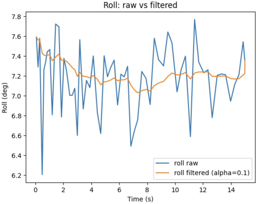
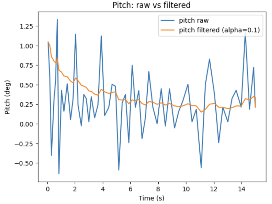
I decided to apply a simple lowpass filter on the data using the equations from class:

$$ \theta_{LPF}[n] = \alpha \cdot \theta_{RAW} + ( 1 - \alpha)*\theta_{LPF}[n-1] $$

$$ \theta_{LPF}[n-1] = \theta_{LPF}[n] $$

$$ \alpha = \frac{T}{T + RC} $$

$$ f_{c} = \frac{1}{2 \pi RC} $$

Task 2 - Gyroscope

For the gyroscope, I used the class equation: $\theta_{g}=\theta_{g}+GyroReading \cdot dt$ to compute pitch, roll, and yaw angles.

unsigned long now_us = micros();
float dt = (now_us - last_us) / 1000000.0f; // seconds
last_us = now_us;
roll_g  += gx * dt;
pitch_g += gy * dt;
yaw_g   += gz * dt;

As you can see below, the gyroscope readings increase over time and drift when not corrected.

I changed the delay(30) (first video) in the loop to delay(10) (second video) as shown below:

After, I added the following complementary filter from class: $\theta = (\theta + \theta_{g})(1-\alpha)+\theta{a} \alpha$ with an $\alpha$ value of 0.6.AAAAAA

float gx = sensor ->gyrX() - gx_bias;
float gy = sensor ->gyrY() - gy_bias;
float gz = sensor ->gyrZ() - gz_bias;

float roll_acc  = atan2(ay, az) * 180.0 / M_PI;
float pitch_acc = atan2(-ax, sqrt(ay*ay + az*az)) * 180.0 / M_PI;

unsigned long now_us = micros();
float dt = (now_us - last_us) / 1000000.0f; // seconds
last_us = now_us;

//  float roll_gyro  = roll_cf  + gx * dt;
//  float pitch_gyro = pitch_cf + gy * dt;

roll_g  += gx * dt;
pitch_g += gy * dt;
yaw_g   += gz * dt;

roll_cf  = alpha * (roll_cf + gx * dt) + (1.0f - alpha) * roll_acc;
pitch_cf = alpha * (pitch_cf + gy * dt) + (1.0f - alpha) * pitch_acc;

As you can see in the video below, the filter reduces the drift, and does not make the data susceptible to quick vibrations or drifts.

The gyroscope's accuracy can be controlled by calibrating the bias at startup with the device being stationary or by selecting a value of $\alpha$ that is suitable for the system. A lower $\alpha$ corrects the acceleration more often.

Task 3 - Sampling Data

I attempted running the IMU and collected the following information from the run: 02:42:47.223 -> DONE CAPTURE 02:42:47.223 -> Samples: 1000 02:42:47.223 -> Avg dt (us): 2695.42 02:42:47.223 -> Estimated fs (Hz): 371.00 02:42:47.223 -> Total loop iterations: 1008 02:42:47.223 -> Max loops between samples: 9

This means that there were about 371 samples per second, and the CPU looped about nine times between samples. Therefore, the main loop runs faster than the IMU produces new values.

This data came running the following code in void loop:

if (recording && (idx < N) && myICM.dataReady()) {
    myICM.getAGMT();

    // timestamp
    t_us[idx] = micros();

    ax[idx] = myICM.accX();
    ay[idx] = myICM.accY();
    az[idx] = myICM.accZ();

    if (loopsSinceLastSample > maxLoopsBetweenSamples)
      maxLoopsBetweenSamples = loopsSinceLastSample;

    loopsSinceLastSample = 0;
    idx++;

    if (idx >= N) stopRecording();
  }

  // printing results once capturing is finished
  if (!recording && idx == N) {
    // Estimate sampling rate from timestamps
    uint32_t dt_sum = 0;
    for (int i = 1; i < N; i++) dt_sum += (t_us[i] - t_us[i-1]);
    float dt_avg_us = dt_sum / float(N - 1);
    float fs = 1e6f / dt_avg_us;

    Serial.println("DONE CAPTURE");
    Serial.print("Samples: "); Serial.println(N);
    Serial.print("Avg dt (us): "); Serial.println(dt_avg_us);
    Serial.print("Estimated fs (Hz): "); Serial.println(fs);
    Serial.print("Total loop iterations: "); Serial.println(loopCount);
    Serial.print("Max loops between samples: "); Serial.println(maxLoopsBetweenSamples);

In order to collect time-stamped values into an array I used the following code:

if (micros() - capture_start_us <=5000000 && myICM.dataReady()){
    myICM.getAGMT();
    float ax = myICM.accX();
    float ay = myICM.accY();
    float az = myICM.accZ();
    
    float gx = myICM.gyrX() - gx_bias;
    float gy = myICM.gyrY() - gy_bias;
    float gz = myICM.gyrZ() - gz_bias;

    float roll_acc  = atan2(ay, az) * 180.0 / M_PI;
    float pitch_acc = atan2(-ax, sqrt(ay*ay + az*az)) * 180.0 / M_PI;
    
    unsigned long now_us = micros();
    float dt = (now_us - last_us) / 1000000.0f; // seconds
    last_us = now_us;
    
    roll_g  += gx * dt;
    pitch_g += gy * dt;
    yaw_g   += gz * dt;

    roll_cf  = alpha * (roll_cf  + gx * dt) + (1.0f - alpha) * roll_acc;
    pitch_cf = alpha * (pitch_cf + gy * dt) + (1.0f - alpha) * pitch_acc;

    float timee = (micros() - capture_start_us)/1e6f;

    roll_acc_arr[loopCount] = roll_acc;
    pitch_acc_arr[loopCount] = pitch_acc;
    roll_gyr_arr[loopCount] = roll_cf;
    pitch_gyr_arr[loopCount] = pitch_cf;
    time_arr[loopCount] = timee;
    idx++;

}

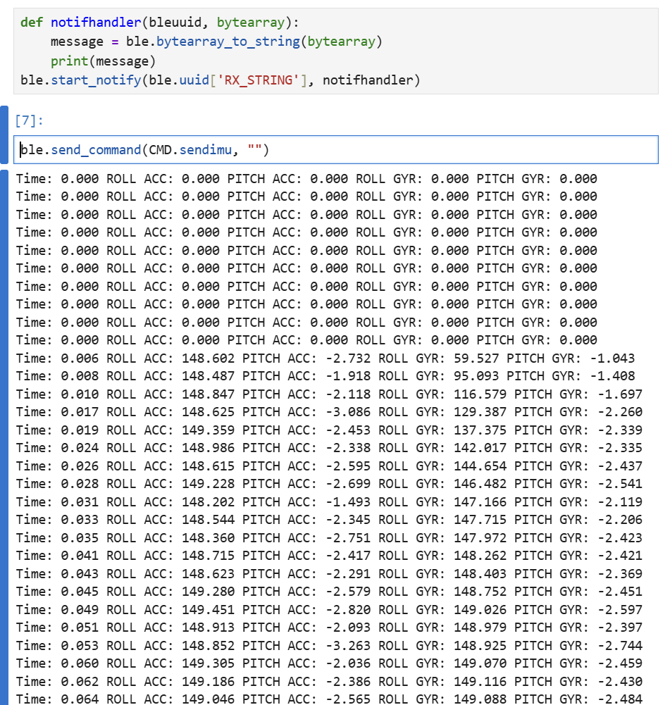
This code captured five seconds worth of data and I sent it over via BLE via the following function:

case sendimu:{  
    for(int i=0; i < idx;i++){
    tx_estring_value.clear(); 
    tx_estring_value.append("Time: ");
    tx_estring_value.append(time_arr[i]);
    tx_estring_value.append(" ROLL ACC: ");
    tx_estring_value.append(roll_acc_arr[i]);
    tx_estring_value.append(" PITCH ACC: ");
    tx_estring_value.append(pitch_acc_arr[i]);
    tx_estring_value.append(" ROLL GYR: ");
    tx_estring_value.append(roll_gyr_arr[i]);
    tx_estring_value.append(" PITCH GYR: ");
    tx_estring_value.append(pitch_gyr_arr[i]);
    tx_characteristic_string.writeValue(tx_estring_value.c_str());
    }
}

and called it in Jupyter via:

ble.send_command(CMD.sendimu, "")

Here is an example of the data sent over:

Overall, I believe it may make most sense to have separate arrays that store different values such as time, accelerometer data, gyroscope data, as it allows to append samples at the same index across signals, and send the data over BLE line-by-line. Floats seem to be the most fast and compact values, compared to strings and doubles.

The RedBoard Artemis Nano has about 384 kB of RAM. This multiplied by 1024 equates to 393,216 bytes. If I send over 5 floats, knowing that each float equates to 4 bytes, then I would be using 20 bytes. The maximum amount of samples that I could store would be 393,216/20 = 19,660.8 samples. Using the values of 371 samples per second from before, this equates to approximately 52.99 seconds.

STUNT!

Unfortunately, when I first plugged in my car, it worked for a few seconds with the remote control and then began only spinning the wheels on one side. It would not receive commands from the control, it would just spin on its own. Because of this I am only able to record one trick of it spinning in place :(.

The following video is of tricks I performed when I was able to borrow a friend's car :).

Resources & Collaborations

I used ChatGPT to help solve the nonzero pitch values as explained above, to help create the frequency graphs in python, and to help write the process in void loop that allowed me to collect data and timestamps to process later on.