Lab 5

Prelab

In this lab, I implement PI control using the ToF sensor data to maintain the car 1 ft (304mm) away from a wall when driving the car as fast as possible.

To complete this goal, there are a number of supporting cases and flags that I created to be able to run things smoothly over BLE without risk of losing control of the car.

The cases that I would use for each run are PI_POS, STOP_CAR, and SEND_DATA.

The PI_POS case sets up all variables and flags necessary for the PI_POS() function to run in the main loop.

case PI_POS:{
    float p_gain;
    float i_gain;
    success = robot_cmd.get_next_value(p_gain);
    if (!success)
    return;
    success = robot_cmd.get_next_value(i_gain);
    if (!success)
    return;
    prop_gain = p_gain;
    int_gain = i_gain;
    integral = 0;
    last_pi_ms = millis();
    ext_number = 0;        
    last_tof_time = 0;
    prev_tof_time = 0;
    loop_samplecount = 0;
    samplecount = 0;
    tof_front.startRanging();
    while(!tof_front.checkForDataReady()) delay(1);
    last_tof_reading = tof_front.getDistance();      
    last_tof_reading_ext = last_tof_reading;
    pi_run = true;
    break;
}    

Setting pi_run to true means that the PI_POS() function runs in the main loop:

void loop(){
    ...
    if(pi_run){
      PI_RUN();
      }
}

In order to stop the run I would send the STOP_CAR command over BLE which runs this switch case:

case STOP_CAR:{
    pi_run = false;
    tof_front.stopRanging();
    hardStop();
    break;
}

The hardStop() function sets all four motor driver pins(including forward and reverse simultaneously) to 255.

The PI_RUN() function collects data throughout the run. Once the run is over I would send data over to my computer by running the following command over BLE:

case SEND_DATA:{
for (int i=0; i<samplecount;i++){  
    tx_estring_value.clear(); 
    tx_estring_value.append("Time (ms): ");
    tx_estring_value.append((int)time_array[i]);       
    tx_estring_value.append(", Front (mm): ");
    tx_estring_value.append((int)toffront_array[i]);
    tx_estring_value.append(", Motor PWM: ");
    tx_estring_value.append((int)motor_out_array[i]);
    tx_estring_value.append(", Extrapolated (mm): ");
    tx_estring_value.append((int)extr_array[i]);
    tx_characteristic_string.writeValue(tx_estring_value.c_str());
    }
    break;
}

On the Jupyter lab side I'd send the commands using the following lines of code:

ble.send_command(CMD.PID_POS, "0.23|0.013")
ble.send_command(CMD.STOP_CAR, "")
ble.send_command(CMD.SEND_DATA, "")

The values in the PID_POS command represent the proportional and integrator gains respectively.

Task 1 - ToF Sensor Sampling Frequency

To begin, I wanted to measure the frequency that the ToF returns new data.

def notifhandler(bleuuid, bytearray):
    message = ble.bytearray_to_string(bytearray)
    print(message)    
ble.start_notify(ble.uuid['RX_STRING'], notifhandler)
ble.send_command(CMD.COLLECT_DATA, "")
ble.send_command(CMD.SEND_DATA, "")

I collect the code using the following loop in the COLLECT_DATA case:

while(millis() - startMillis < sampletime){
          if(tof_lat.checkForDataReady() && tof_front.checkForDataReady() ){
            toflat_array[samplecount] = tof_lat.getDistance();
            toffront_array[samplecount] = tof_front.getDistance();
            tof_lat.clearInterrupt();
            tof_front.clearInterrupt();
            time_array[samplecount] = millis();
            samplecount++;    
          }
      }

Then I sent it over in the SEND_CASE case:

for (int i=0; i<samplecount;i++){  
          tx_estring_value.clear(); 
          tx_estring_value.append("Time (ms): ");
          tx_estring_value.append((int)time_array[i]);       
          tx_estring_value.append(", Front (mm): ");
          tx_estring_value.append((int)toffront_array[i]);
          tx_estring_value.append(", Lateral (mm): ");
          tx_estring_value.append((int)toflat_array[i]);
          tx_characteristic_string.writeValue(tx_estring_value.c_str());
          }

And received the following output:

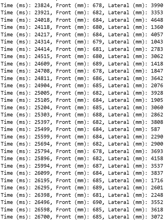
The average time between each data sample is 99.2 ms, wich equates to roughly 10 Hz.

I attempted rerunning this after having changed the timing budget of the ToF sensors to 20 ms. This reduces the accuracy of the readings, therefore, I decided to set the sensors to Short Mode. This made the most sense to me, as we want to reach within 1 ft of the wall, and the maximum distance in this mode is ~4.3 ft.

    tof_front.setTimingBudgetInMs(20);
    tof_front.setIntermeasurementPeriod(20);
    tof_lat.setTimingBudgetInMs(20);
    tof_lat.setIntermeasurementPeriod(20);    

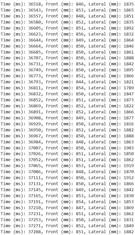
Now, there was much more data outputted, with a frequency of about 48 Hz.

Task 2 - Calculating PI

Now I decided to calculate the PI control, and decouple it from ToF readings, such that the loop runs regardless of whether or not data from the ToF sensors was received. The PI control will take in measurements from the ToF sensors, however, if the data is not ready in time then the new PI values are calculated based on the previous ToF sensor values. For the rest of this lab, the only ToF data that will be used will be from the front sensor.

I began with only proportional control, then introduced integral. I decided to not implement derivative control into the system, as derivative control amplifies noise and the ToF sensor is noisy enough. To determine the proportional gain value I used the formula:

$$ PWM Signal = K_{p} (Target Position - Actual Position) $$

$$ K_{p} = \frac{\Delta Output}{\Delta Error} $$

Knowing that we want our output to be ~304 mm, and that the maximum that our error could ever be is 1300mm (max sensor output), I started off with a gain of 0.23.

I decided to have a series of flags that the code relied on to run the PI control. The flags are updated by the functions being run, or from cases that I would run via BLE.

ble.send_command(CMD.PI_POS, 0.23)

case PI_POS:{
        float p_gain;
        success = robot_cmd.get_next_value(p_gain);
        if (!success)
        return;
        samplecount = 0;
        tof_front.startRanging();
        prop_gain = p_gain;
        pi_run = true;
        break;
       }

This causes a flag in the main void loop () to turn true and runs this function:

void PI_RUN(){
    float target = 304.0;

    if (tof_front.checkForDataReady()){
        last_tof_reading = tof_front.getDistance();
        tof_front.clearInterrupt();

        if(samplecount < samplesize){
            toffront_array[samplecount] = last_tof_reading;
            time_array[samplecount] = millis();
            samplecount++;
        }
    }

    float error = last_tof_reading - target;

        if(abs(error) < 20){
        hardStop();
        tof_front.stopRanging();
        tx_estring_value.clear(); 
        tx_characteristic_string.writeValue("Within target range");
        data_collected = true;
        pi_run = false;
        }

    int pwm = prop_gain * error;
    pwm = constrain(pwm, -255, 255);

    if(pwm>0){
        forward(abs(pwm), 0);
    }
    else if(pwm<0){
        reverse(abs(pwm), 0);
    }

}

I decided to leave a tolerance of about 20mm (6.5%).

Running this gave me the following output:

As you can see, the car never reaches the target value.

Now, I decided to add in an integrator gain. I chose this value by going off of the proportional gain value and dividng it by an integrating time of ~20s I ended up with a value of 0.013. I added in global variables, int_gain, and integral, and last_pi_ms.

Updated the case:

case PI_POS:{
        float p_gain;
        float i_gain;
        success = robot_cmd.get_next_value(p_gain);
        if (!success)
        return;
        success = robot_cmd.get_next_value(i_gain);
        if (!success)
        return;
        
        prop_gain = p_gain;
        int_gain = i_gain;
        integral = 0;
        last_pi_ms = millis();
        samplecount = 0;
        tof_front.startRanging();
        pi_run = true;
        break;
       }

And updated the PI_RUN() function by adding these lines:

unsigned long now_ms = millis();
float dt = (now_ms - last_pi_ms) / 1000.0f;
last_pi_ms = now_ms;
integral += error * dt;
int pwm = (prop_gain * error) + (int_gain * integral);

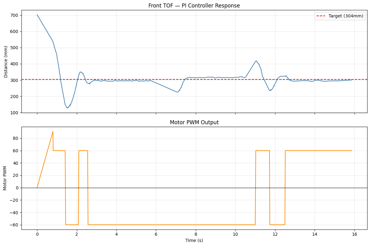
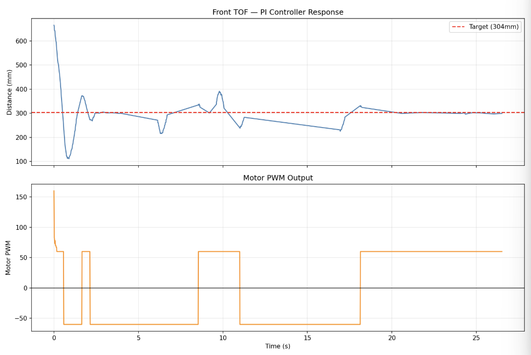
Here is the run:

From the following output we can see how the car managed to reach the target goal, with initial overshoot. The later deviations are from pushing the car and it correcting itself.

Task 3 - Determining Speed of PI Control Loop

I added in a separate array and counter to track how often the PI control loop runs:

float loop_time_arr[samplesize];
int loop_samplecount = 0;
unsigned long last_loop_ms = 0;

Started logging within the PI_RUN() function:

unsigned long now = millis();
if(loop_samplecount<samplesize){
    loop_time_arr[loop_samplecount] = now - last_loop_ms;
    loop_samplecount++;
}
last_loop_ms = now;

And added in the data to the SEND_DATA case:

for(int i=0; i<loop_samplecount; i++){
    tx_estring_value.clear();
    tx_estring_value.append("Loop dt (ms): ");
    tx_estring_value.append((int)loop_time_arr[i]);
    tx_characteristic_string.writeValue(tx_estring_value.c_str());
}

This would output:

Averaging all of the times (ignoring the spikes due to write_data() sending BLE packets every 500 ms) gives an average dt of 9.1 ms, which equates to ~110Hz. This is nearly twice as fast as the ToF sensor data, meaning that at least half of the time the PI loop is running based on an expired value.

Task 4 - Extrapolating an Estimated Distance

Instead of using the previous datapoint to calculate the necessary PWM value, I'll extrapolate an estimate for the car's distance to the wall using the amount of time that has passed, and the slope between the two most recent datapoints.

//extrapolation variables:
unsigned long last_tof_time = 0;
unsigned long prev_tof_time = 0;

I decided to do this by adding the following code in the PI_RUN() function:

if (tof_front.checkForDataReady()){
      last_tof_reading_ext = last_tof_reading;
      prev_tof_time = last_tof_time;
      last_tof_reading = tof_front.getDistance();
      last_tof_time = millis();
      tof_front.clearInterrupt();
      ext_number++;
      ...
    }

And added:

float estimated_pos = last_tof_reading;

if(ext_number > 1){
float sensor_dt = last_tof_time - prev_tof_time;  // ms between last two readings
if(sensor_dt > 0){
    float slope = (last_tof_reading - last_tof_reading_ext) / sensor_dt;  // mm/ms
    float time_since_last = millis() - last_tof_time;  // ms since last reading
    estimated_pos = last_tof_reading + slope * time_since_last;
    }
}
float error = estimated_pos - target;

Lastly, I added these to the PI_POS case to reset the variable for every time I want to run PI control:

ext_number = 0;        
last_tof_time = 0;
prev_tof_time = 0;
tof_front.startRanging();
while(!tof_front.checkForDataReady()) delay(1);
last_tof_reading = tof_front.getDistance();      
last_tof_reading_ext = last_tof_reading; 

Here's a video of the run with the extrapolation taking place:

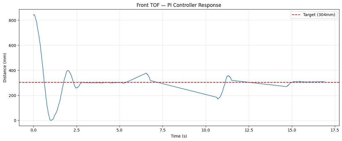
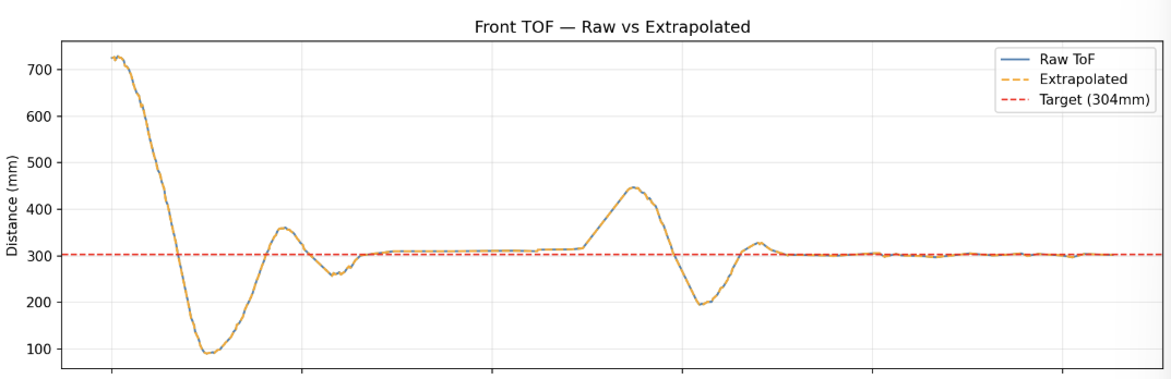
Here is data from a second run:

Here is a another graph of the Raw ToF data compared to the extrapolated data. As you can see, there is not much differene between the two. I believe this is due to the quite rate that I set the ToF to generate data with.

5000-level Task - Wind-Up Protection

With no wind-up protection, the integrator term accumulates unboundedly. If the value grows too large, the error can cause the controller to run the motors at full power regardless of the position it is at. This is a great cause for concern, as the only way to correct this is unwinding in the opposite direction. Therefore, I constrained the integral to not exceed -500 or 500, which intentionally gives the integrator small weight on the PWM control, as I only wish to use it to correct the residual steady-state error that the P term cannot overcome. With a Ki of 0.013, the maximum PWM that it can contribute is 6.5 (0.013*500).

integral += error * dt;
integral = constrain(integral, -500, 500); 

With wind-up protection:

Without:

With wind-up correction: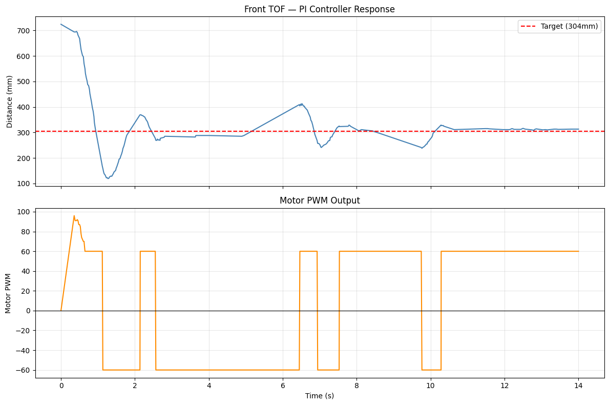

Without wind-up correction: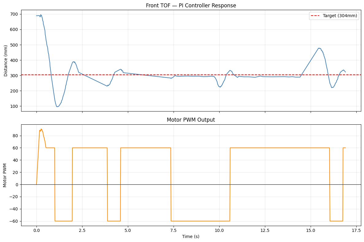

Added Videos of More Runs:

As for speed, the maximum linear speed observed came from logged sensor data where the car dropped 122 mm in 125 ms, which comes out to a speed of 0.98 m/s.