Lab 6

Prelab

In this lab I will be implementing PID control to control the orientation of the stationary car. Digital integration may lead to yaw drift, as the gyroscope accumulates small errors over time, even when the robot is stationary. For this reason, I will be using the IMU's Digital Motion Processing (DMP) which uses a sensor fusion algorithm that accounts for this and performs calibrations when encessary.

The gyroscope has a typical bias of about +/- 3 dps, which means that over 10 seconds, a drift of 30 degrees may accumulate. The DMP corrects for this on the IMU directly.

The gyroscope is rated for the following range of rotational velocities: +/- 250 dps, +/- 500 dps, +/- 1000 dps, and +/- 2000 dps. At +/- 250 dps, the robot can complete an entire 360 in about 1.4 seconds, which is plenty of time considering our car will be making small, corrective turns. For future needs, I can configure this in the library.

To access the yaw value using DMP I defined it early on in my code and used the following in the actual control functions PID_ANGLE:

    icm_20948_DMP_data_t data;
    do {
        myICM.readDMPdataFromFIFO(&data);
    } while (myICM.status == ICM_20948_Stat_FIFOMoreDataAvail);

    if ((myICM.status == ICM_20948_Stat_Ok) && (data.header & DMP_header_bitmap_Quat6)) {
        double q1 = ((double)data.Quat6.Data.Q1) / 1073741824.0;
        double q2 = ((double)data.Quat6.Data.Q2) / 1073741824.0;
        double q3 = ((double)data.Quat6.Data.Q3) / 1073741824.0;
        double q0 = sqrt(1.0 - min(1.0, q1*q1 + q2*q2 + q3*q3));

        // Extract yaw
        yaw_g = atan2(2.0*(q0*q3 + q1*q2), 1.0 - 2.0*(q2*q2 + q3*q3)) * 180.0 / M_PI;
    }

For this lab, I plan on sending and receiving data a bit differently to how I would in Lab 5. This is because of the nature of the controller, where I would like to receive data as the program itself is running. This will be useful in later labs when I would like to see real-time data.

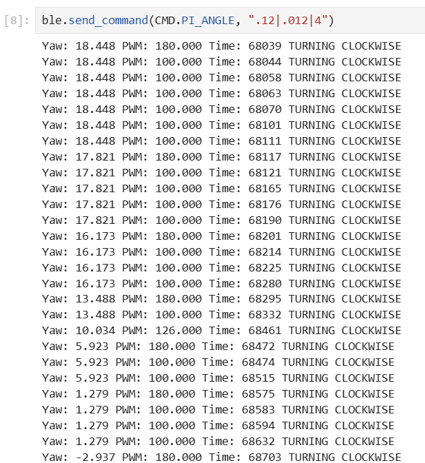
I did this by sending the values over BLE inside of the control function. For example here is what I have for when the car must turn clockwise:

if(error < 0){
    oneaxisCCW(abs(pwm),0);
    tx_estring_value.clear();
    tx_estring_value.append("Yaw: ");
    tx_estring_value.append((float)yaw_g);
    tx_estring_value.append(" PWM: ");
    tx_estring_value.append((float)pwm);
    tx_estring_value.append(" Time: ");
    tx_estring_value.append((int)millis());
    tx_estring_value.append(" TURNING COUNTERCLOCKWISE");
    tx_characteristic_string.writeValue(tx_estring_value.c_str());        
    }

This way I am constantly receiving data and am not limited to an array that is constrained in size and possible does not capture the entire run:

I was able to control the car via BLE in order to start and stop runs and collect data using the following code:

ble.send_command(CMD.PI_ANGLE, ".12|.012|4")
ble.send_command(CMD.STOP_CAR, "")

The current implementation only drives motors in opposite directions for rotation. To support orientation control while driving, the motor outputs would need to be decomposed into a forward velocity component and a differential yaw correction component.

Task 1 - Implementing P Control

The DMP is configured to output at approximately 10 Hz.

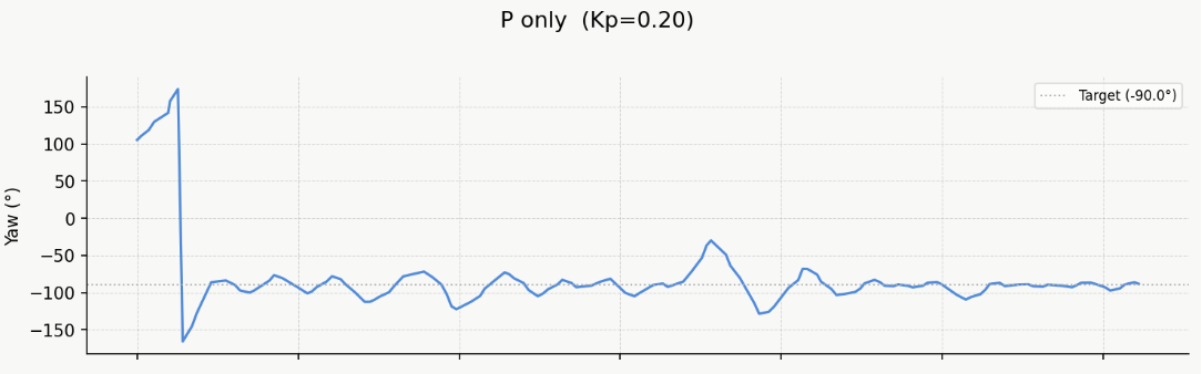
To begin, I started implementing proportional control the same way that I did for Lab 5, however, this lab required a more empirical approach to reach the final value. I started off determining the Kp value just as I did for Lab 5 using the following equation: $$PWM = K_p \cdot e(t), \quad e(t) = \text{target} - \text{yaw}$$ where the error is wrapped to ±180°. I selected a target angle of 90 degrees, therefore I estimated that the maximum error at the start of a turn would be around 90° and selecting Kp such that Kp × 90 fell near the middle of the usable PWM range (100–180). This gave a Kp of ~2. I then tuned downward empirically from there, as originally, the car would vastly overshoot and undershoot, leading me to settle on Kp = 0.2.

I performed this proportional gain control using similar code to what I used for Lab 5 with a few adjustments:

float error = fmod(target - yaw_g + 540.0, 360.0) - 180.0;
pwm = (prop_gain * error)

if(error > 0){
        oneaxisCW(abs(pwm),0);
        tx_estring_value.clear();
        tx_estring_value.append("Yaw: ");
        tx_estring_value.append((float)yaw_g);
        tx_estring_value.append(" PWM: ");
        tx_estring_value.append((float)pwm);
        tx_estring_value.append(" Time: ");
        tx_estring_value.append((int)millis());
        tx_estring_value.append(" TURNING CLOCKWISE");
        tx_characteristic_string.writeValue(tx_estring_value.c_str());
        //Serial.println("TURNING CLOCKWISE");
    }

if(error < 0){
    oneaxisCCW(abs(pwm),0);
    tx_estring_value.clear();
    tx_estring_value.append("Yaw: ");
    tx_estring_value.append((float)yaw_g);
    tx_estring_value.append(" PWM: ");
    tx_estring_value.append((float)pwm);
    tx_estring_value.append(" Time: ");
    tx_estring_value.append((int)millis());
    tx_estring_value.append(" TURNING COUNTERCLOCKWISE");
    tx_characteristic_string.writeValue(tx_estring_value.c_str());        
}

I decided to add a tolerance of about 3 degreees to give the system clearance.

Task 2 - Implementing PI Control

For the integral control I determined Ki empirically, beginning with a Ki = Kp/10 = ~0.02. This soon was reduced to 0.012 after observing that the integral term accumulated too aggressively during the initial large-error phase. I added the following code to the control function:

integral += error * dt;
pwm = (prop_gain * error) + (int_gain * integral)

And I added this to the switch case:

case PI_ANGLE:{
        float p_gain;
        float i_gain;
        success = robot_cmd.get_next_value(p_gain);
        if (!success)
        return;
        success = robot_cmd.get_next_value(i_gain);
        if (!success)
        return;
        prop_gain = p_gain;
        int_gain = i_gain;
        integral = 0;
        last_pi_ms = millis();
        samplecount = 0;
        pi_run = true;
        break;
       }

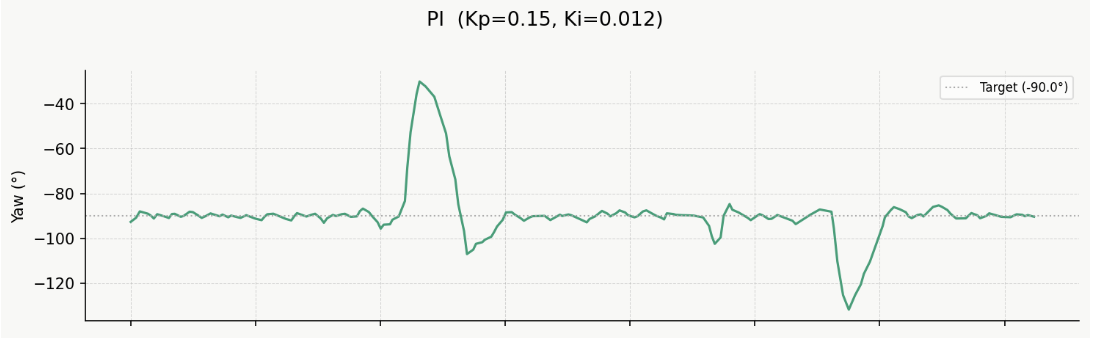
You can see how the system still oscillates about the target value, but never stays stable. For this reason, I decided to introduce derivative control.

Task 3 - Implementing PID Control

Derivative kick comes from a sudden change in setpoint that produces a large spike in the derivative term, since the error jumps intantaneously. For this lab, I take the derivative of the error and not a measurement, meaning that it would produce a kick. However, for this lab, the setpoint is set to 90 degrees, so it is not an issue. In the future, for applications that will contain sudden setpoint changes I may switch to take the derivative of measurements: $$\frac{yaw_{now} - yaw_{prev}}{dt}$$.

Taking the derivative of a gyroscope-integrated signal gives us the angular velocity. However, in this lab I am relying on DMP capabilities instead of having the Artemis manually calculate the values.

A low-pass filter on the derivative was not implemented. The DMP output is already smooth, and does not cause noise amplification that can cause concern for derivative terms. I did not observe excessive jitter or isuees with large Kd values, making a low-pass filter not necessary.

Finally, in order to add the derivative control term I added in the following code to the case and function itself:

case PI_ANGLE:{
        ...
        float d_gain;
        success = robot_cmd.get_next_value(d_gain);
        if (!success)
        return;
        der_gain = d_gain;
        prev_error = 0;
        ...
        break;
       }

float derivative = (dt > 0) ? (error - prev_error) / dt : 0.0f;
prev_error = error;
...
pwm = (prop_gain * error) + (int_gain * integral) + (der_gain * derivative);;
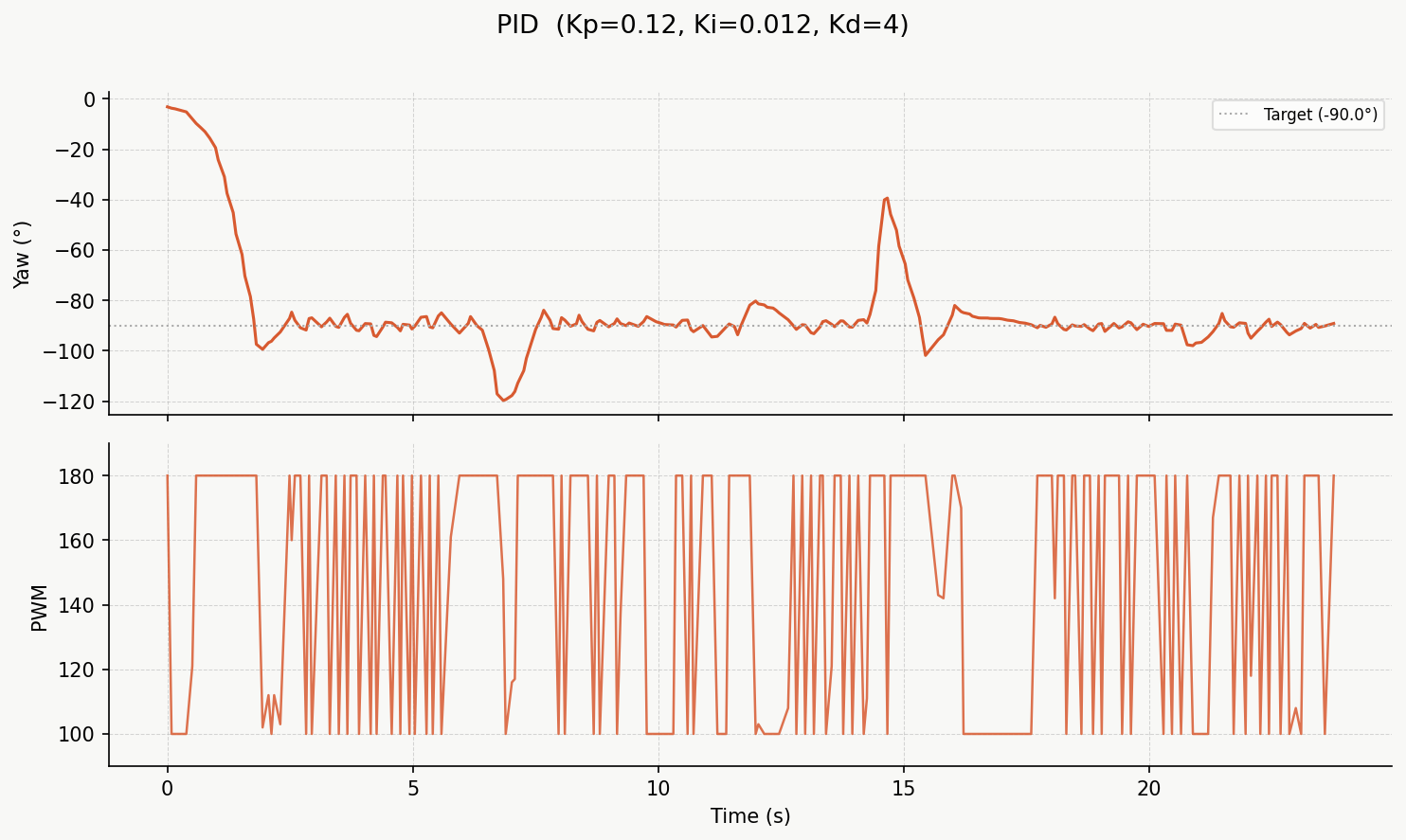
pwm = constrain(abs(pwm), 100, 180);

I constrained the pwm values, such that the motors would have enough power to overcome static friction, and that it would not be large enough to drastically overshoot the target value.

I believed that adding the derivative term would help entirely eliminate the oscilliation, however, unfortunately it did not. I decided to increase the derivative gain as much as possible, but did not want to exagerate and introduce noise and discrepancies into the system.

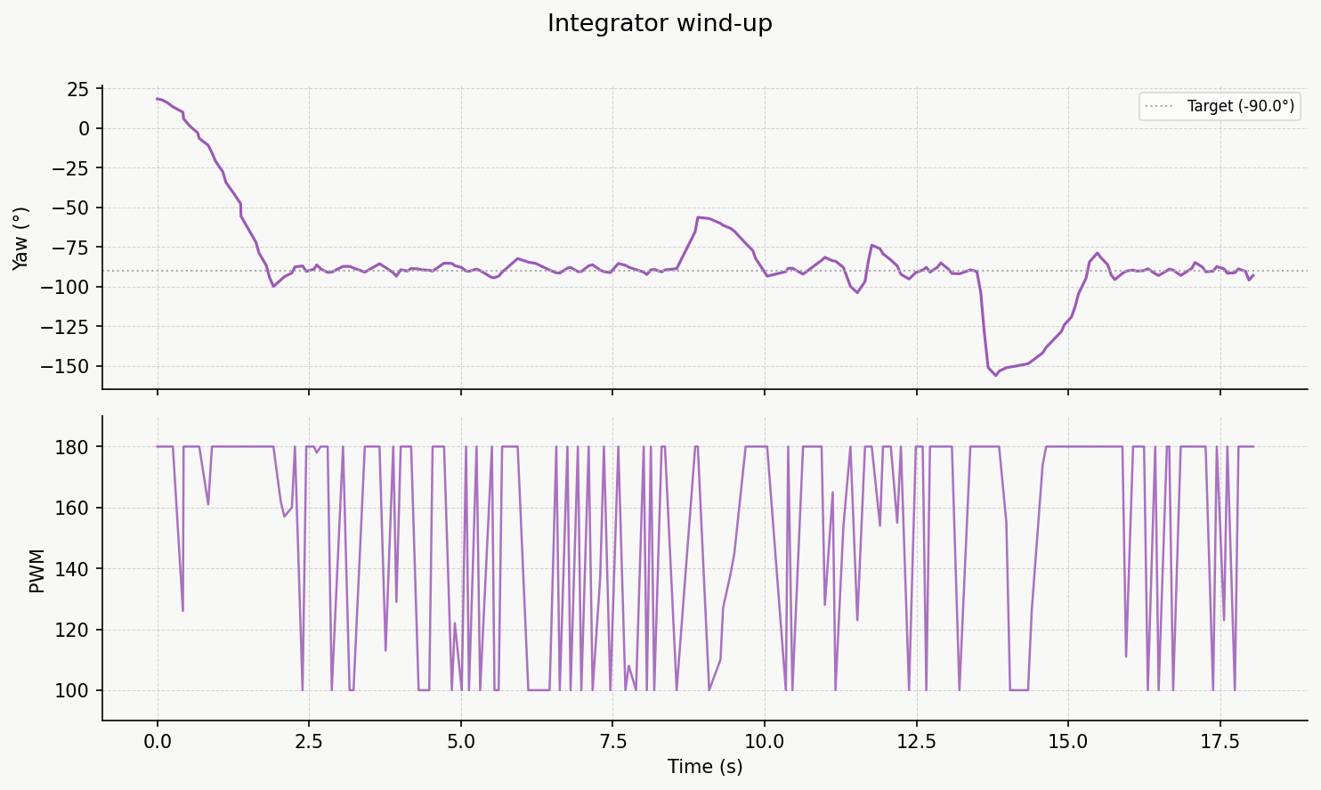
5000-Level Task

Wind-up protection is important for the integral control, for the same reasons in this lab as they are for Lab 5. It is important for the integral to not grow unboundedly, and in order to do this I decided to constrain it using the following code:

Ki * integral must not exceed 255, given that this value is the maximum pwm signal that is configured for our motors. $$integral <= \frac{255}{K_{i}}$$, and with Ki being 0.012, I chose the following bounds:

integral = constrain(integral, -21250, 21250);

References & Reflection

I was out of town, therefore did not have the batteries that fit the car and had to hold them to perform the runs. I decided to add duct tape to the wheels, as the wheels' grip made it difficult for the car to simulateneously run the wheels forwards and backwards on each side.

I used Claude in order to help me integrate DMP into my code and it helped me generate the following code that I used in my setup:

bool imu_ready = false;
while (!imu_ready) {
  myICM.begin(WIRE_PORT, AD0_VAL);
  if (myICM.status == ICM_20948_Stat_Ok) {
    imu_ready = true;
  } else {
    Serial.println("IMU not ready, retrying...");
    delay(500);
  }
}
Serial.println("IMU connected!");

bool success = true;
success &= (myICM.initializeDMP() == ICM_20948_Stat_Ok);
success &= (myICM.enableDMPSensor(INV_ICM20948_SENSOR_GAME_ROTATION_VECTOR) == ICM_20948_Stat_Ok);
success &= (myICM.setDMPODRrate(DMP_ODR_Reg_Quat6, 4) == ICM_20948_Stat_Ok); // ~10Hz, safe for BLE loop
success &= (myICM.enableFIFO() == ICM_20948_Stat_Ok);
success &= (myICM.enableDMP() == ICM_20948_Stat_Ok);
success &= (myICM.resetDMP() == ICM_20948_Stat_Ok);
success &= (myICM.resetFIFO() == ICM_20948_Stat_Ok);
if (!success) { Serial.println("DMP init failed!"); while(1); }