Lab 7
Prelab
In this lab we will be implementing a Kalman Filter into our car. We will repeat Lab 5, however this time we will supplement the sampled ToF values to speed towards the wall as fast as possible, and then stop 1ft away from it or turn within 2ft.
We will have to create a state space model for a system from the following series of equations where $u$ is the motor input (motor force) and $x$ is the car's traveled distance:
$$ F = ma = m\ddot{x} \\ F = u - d\dot{x} \\ m\ddot{x} = u - d\dot{x} \\ \ddot{x} = \frac{u}{m} - \frac{d}{m}\dot{x} $$
$$ A = \left[\begin{matrix} 0 & 1 \\ 0 & \frac{-d}{m} \end{matrix}\right] $$
$$ B = \left[\begin{matrix} 0 \\ \frac{1}{m} \end{matrix}\right] $$
$$ \left[\begin{matrix} \dot{x} \\ \ddot{x} \end{matrix}\right] = A\left[\begin{matrix} x \\ \dot{x} \end{matrix}\right] + Bu $$
Task 1 - Estimating drag and momentum
We will need to estimate the drag and momentum terms for our A & B matrices. I will do this by running the car at constant motor input, and solving for $d$ using: $d = \frac{u_{ss}}{\dot{x_{ss}}}$. And for $m$ using: $m=\frac{-d \cdot t_{0.9}}{ln(1-0.9)}$ I will begin by running the motors at a PWM of 125, which is about 50% of the maximum PWM.
I chose a step time of about 1.5 seconds, since all the runs in Lab 5 were able to reach steady state in under 3 seconds, and the car takes less than 2 seconds to reach the wall when starting about 3 meters from it. Note: for this run I set the sensor to Long Mode and switched the timing budget to 50 ms since the car will be starting about 3m from the wall. For this first run, I ran the following code in JupyterLab:
ble.send_command(CMD.SET_MODE, "Long")
ble.send_command(CMD.START_CAR, "125|0")
await asyncio.sleep(1.5)
ble.send_command(CMD.STOP_CAR, "")
ble.send_command(CMD.SEND_DATA, "")
I added in the delay on the python side, since adding the delay in the switch case would cause BLE to disconnect. The following cases were triggered:
 case COLLECT_DATA: {
    samplecount = 0;
    tof_front.startRanging();
    data_collect = true;
    break;
    }

case START_CAR:{
    float pwm;
    float timee;
    success = robot_cmd.get_next_value(pwm);
    if (!success)
    return;
    success = robot_cmd.get_next_value(timee);
    if (!success)
    return;
    forward(pwm,timee);
    break;
}

case STOP_DATA: {
    data_collect = false;
    tof_front.stopRanging();
    break;
}
First run:
The floor that the robot was running on was pretty uneven, and it was difficult to get good ToF data.
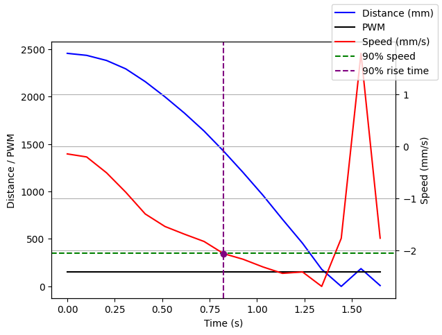
Steady state speed: ~2.2 m/s 90% rise time: ~0.82s Speed at 90% rise time: ~2 m/s
Assuming U is 1N, we can compute:
$$ d = \frac{1 N}{2.2 m/s} = 0.4545 kg/s $$
$$ m = \frac{-0.4545kg/s \cdot 0.82s}{ln(1-0.9)} = 0.162 $$
Task 2 - Initializing Kalman Filter
Now to compute the A and B matrices:
$$ A = \left[\begin{matrix} 0 & 1 \\ 0 & -2.8 \end{matrix}\right] $$
$$ B = \left[\begin{matrix} 0 \\ 6.17 \end{matrix}\right] $$
Although I had set the timing budget to 50ms, the ToF's sensor's sampling time averages ~.103 seconds. Therefore, I begin by using this value to discretize my A and B matrices with the following equations: $A_{d}= I + \Delta T \cdot A$ and $B_{d} = \Delta T \cdot B$.
Manually doing so gives these results:
$$ A_{d} = \left[\begin{matrix} 1 & 0.103 \\ 0 & 0.7116 \end{matrix}\right] $$
$$ B_{d} = \left[\begin{matrix} 0 \\ 0.6355 \end{matrix}\right] $$
However I plugged the following code into Jupyter Lab:
Ad = np.eye(2) + delta_T * A
Bd = delta_T * B
N is the dimension of the state space, which in this case is 2. The C and D matrices will be the following, and the negative comes from the fact that the car will be traveling towards the wall.
$$ C = \left[\begin{matrix} -1 \\ 0 \end{matrix}\right], \ D = \left[\begin{matrix} 0 \\ 0 \end{matrix}\right] $$
I then initialized the state vector:
x = np.array([[-TOF[0]],
              [0]])
where TOF is the ToF data from the first wall against the wall.
To process sensor and general noise I use the following equations from lecture:
$$ \sigma_{1} = \sigma_{2} = 10 \cdot \sqrt{\frac{1}{\Delta T}}\\ \sigma_{3} = 20 mm $$
sig_u=np.array([[sigma_1**2,0],[0,sigma_2**2]])
sig_z=np.array([[sigma_3**2]])
sigma = np.array([[sigma_1**2, 0         ],
                  [0,          sigma_2**2]])
Task 3 - Implementing & Testing Kalman Filter in Python
To check the parameters I implemented my Kalman Filter into the provided python function.
Using the previous code and the provided function I looped through the data using the Kalman Filter at each step:
kf_pos  = []
kf_vel  = []

for i in range(len(front_list)):
    y = np.array([[-front_list[i]]]) #since the distance decreases
    mu, Sigma = kf(mu, Sigma, u_input, y)
    kf_pos.append(mu[0, 0])
    kf_vel.append(mu[1, 0])
And graphed the results:
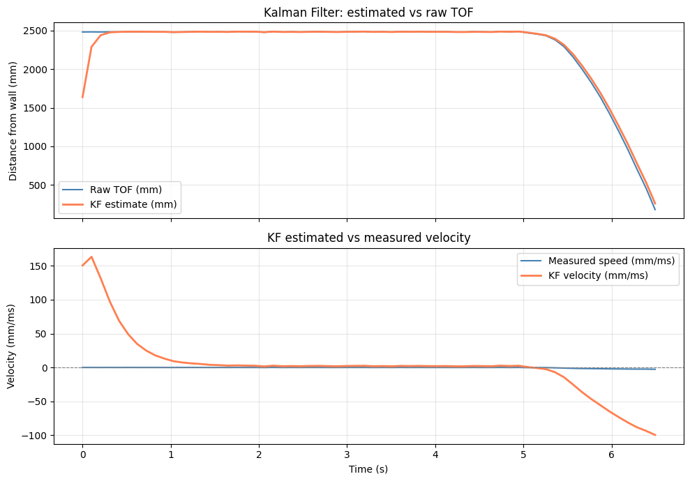
The filter accurately predicted the data, however, deviated at the start and end of the run for the calculated velocity. The initial KF velocity spikes due to a large initial covariance matrix.
There is some discrepancy once the car starts approaching the wall. To fix this, I increased sigma_1 and sigma_2 from 31 to 50 which brought the velocity estimate closer to the measured values.
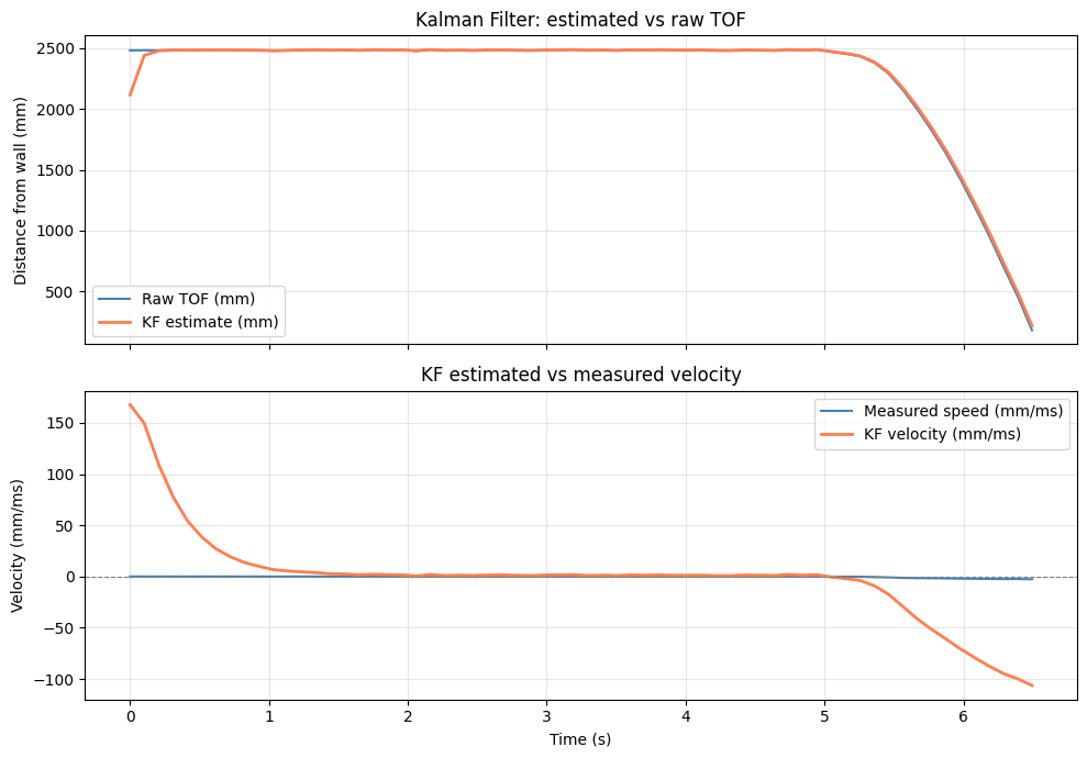
Parameters: Sigma_u (process noise) controls how much the filter trusts the dynamic model. The larger the values is, the more the filter relies on sensor measurements and less on the predicted state. Sigma_z (measurement noise) controls how much the filter trusts the TOF sensor. Larger values make the filter smoother but slower to respond to real changes in distance. Initial state mu — initialized as the first TOF reading with zero velocity. An inaccurate initial state causes transient errors at the start. Initial covariance Sigma — represents confidence in the initial state. A large initial Sigma causes the filter to correct aggressively at first, leading to the velocity spike seen at t=0.
Task 4 - Implementing the Kalman Filter onto the Robot
To implement the Kalman filter into Arduino I defined the state space variables and the variances that were already previously found. And created the following fucntion that would be called upon when running the PI control.
float kf_update(float u_scaled, float y_mm, bool has_meas)
{
    float mp0 = Ad00 * kf_mu0 + Ad01 * kf_mu1;
    ...
    float Sp00 = t00 * Ad00 + t01 * Ad01 + SIG1_SQ;
    float Sp01 = t00 * Ad10 + t01 * Ad11;
    float Sp11 = t10 * Ad10 + t11 * Ad11 + SIG2_SQ;

    if (!has_meas) {
        kf_mu0 = mp0;
        ...
        return kf_mu0;
    }

    float sigma_m = Sp00 + SIG3_SQ;
    float K0 = Sp00 / sigma_m;
    float K1 = Sp01 / sigma_m;
    float innov = y_mm - mp0;
    kf_mu0 = mp0 + K0 * innov;
    kf_mu1 = mp1 + K1 * innov;
    kf_P00 = (1.0f - K0) * Sp00;
    kf_P01 = (1.0f - K0) * Sp01;
    kf_P11 = Sp11 - K1 * Sp01;
    return kf_mu0;
}
And I added this to the PI_RUN() function:
    float u_scaled = -(float)pwm / KF_step;
    float kf_estimated_pos = kf_update(u_scaled, last_tof_reading, has_new_tof);
such that the error uses the KF approximation.
I ended up changing the variance values back to 31, and had to decrease the proportional gain to 0.07 and the integral gain to 0.013.
The result is the following:
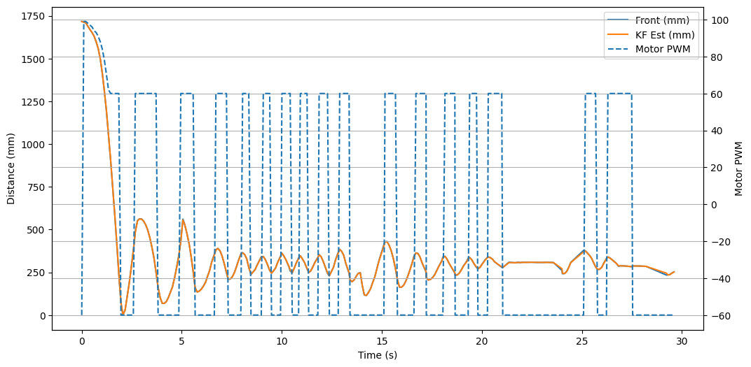
As you can see, the Kalman Filter was surprisingly very accurate with the ToF readings, however, would originally overshoot which led to a lot of bumps against the wall.
References
For this lab, I sourced the equations from the Lecture Slides 'KF (cont), Local Planners', and used Lucca Correia's slides as a reference. Additionally, I used Claude to help implement the Kalman Filter into the robot in c++. This includes aiding with the manual scalar operations and formation of the kf_update function.